Deep Autoencoder Demo - Iteration

Loading this demo takes longer (about 15-20 seconds) than the others.

This is part 2.5 of the series on autoencoders. To know what is happening here, read part 1 and part 2.

In the last two parts on autoencoders, you learned about the two components of an autoencoder: the encoder and the decoder. In the part on decoders, you learned that the decoder's reconstructions are rarely perfect. In this demo, we explore the consequences of the decoder's imperfect ability to reconstruct the image fed into the encoder.

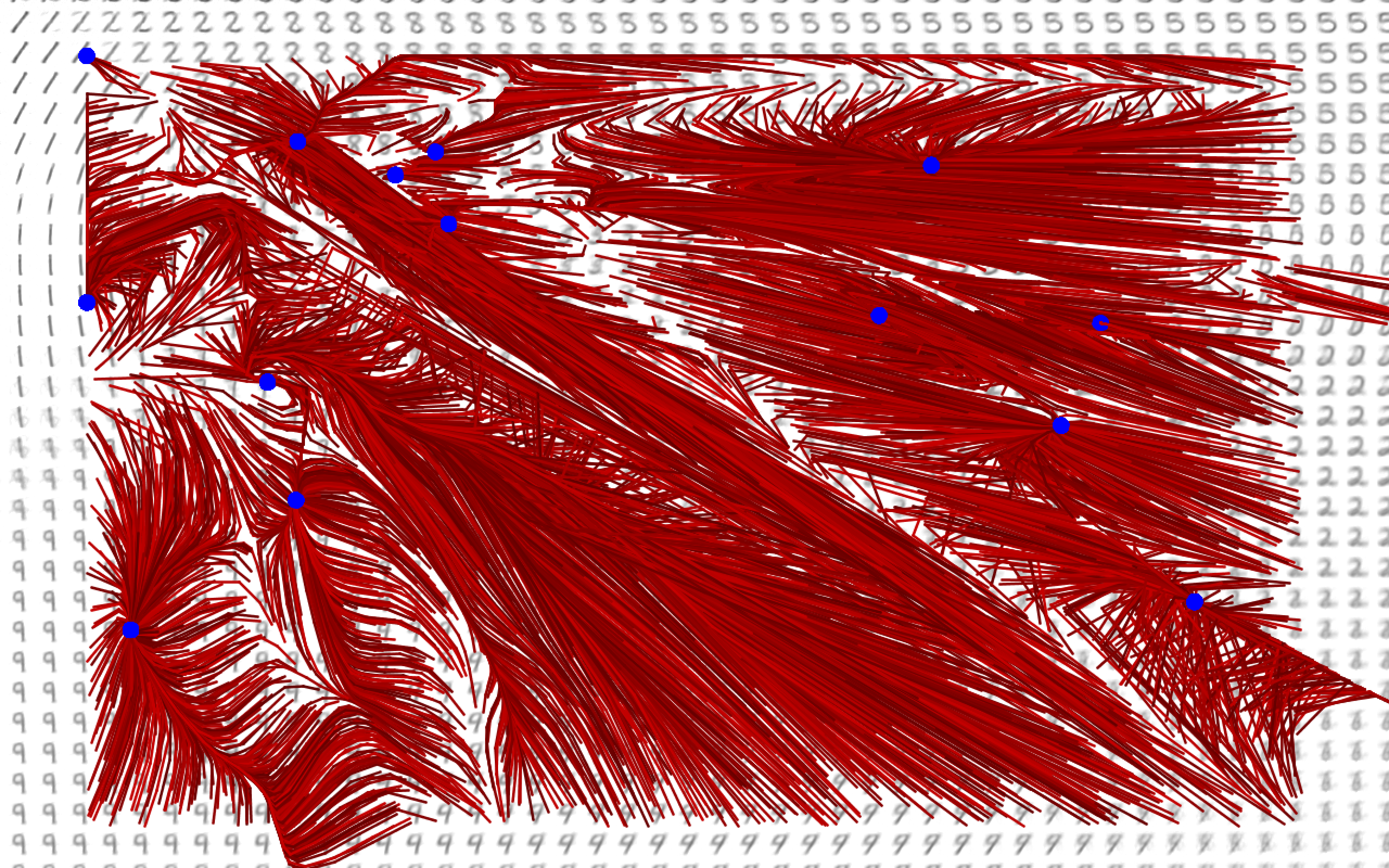
Here is how the demo works: first, a 2D point is picked randomly on the screen. Then, that 2D point is fed into the decoder to produce an image. Then, that image is fed into the encoder to produce another 2D point. Since the encoder and decoder do not act exactly the same, this new 2D point will probably be slightly different. This process is repeated with each 2D point being decoded and then encoded to produce a new point. A red line is drawn between the new point and the old point. If the new point is the same as the old point, a blue circle is drawn at that location.

This procedure results in several red paths being drawn which represent the path taken by an image as it is repeatedly encoded and decoded. The blue circles represent points where the encoder and decoder are "in agreement": the decoder's reconstruction is mapped to that point again, so the decoder's reconstruction could be considered perfect at that point. Much like in part 1, this visualization runs slowly in browsers, so here is what it looks like once many paths have been drawn:



As you can see, the paths tend to converge to a few points with perfect reconstructions. In addition, they tend to fall into a few common routes as they make their way to one of those "perfect" points, like the tributaries of a river. If the paths are drawn semi-transparently, then you get a sort of heatmap of the most common routes the points take as they are iterated:



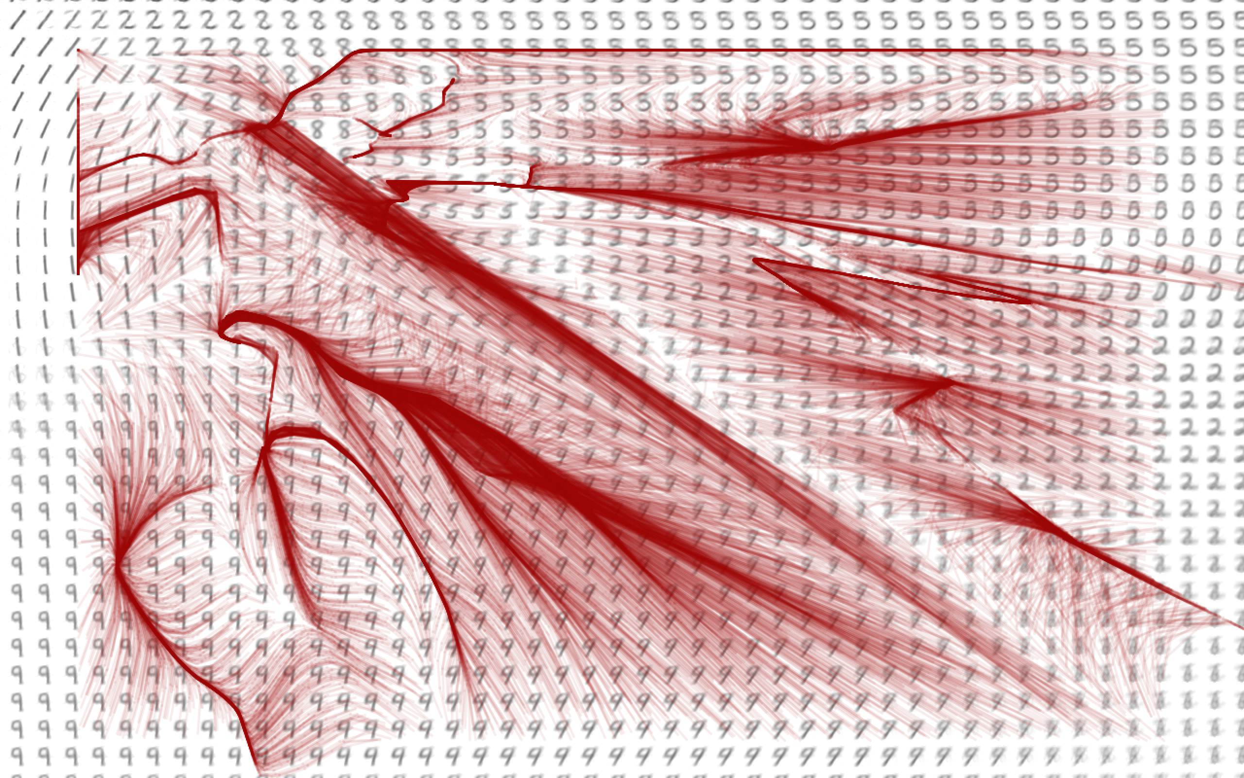
It's very difficult to analyze why exactly these patterns appear, since the autoencoder has tens of thousands of parameters which were learned automatically. However, there is one interesting thing to notice about these paths. If you look closely, you can see that the paths very quickly leave regions with ambiguous images. The biggest example is the diagonal which goes from the top-left of the image to the bottom-right. If you investigate the decoder's reconstructions of those coordinates, you will see that they are nonsensical and don't really look like a particular number. If you look at the paths, you can see that points which find themselves in that region are quickly mapped away from it after another decoder-encoder iteration. This indicates that the encoder tends to map images to non-ambiguous locations. When given an image, it is more likely to map that image to a region where the decoder will be able to make sense of it, rather than a region where the decoder would produce a nonsense reconstruction. If you remember the training procedure from part 1, you might recognize that this fulfills the autoencoder's goal of creating accurate reconstructions. This results in the points tending towards relatively unambiguous locations.

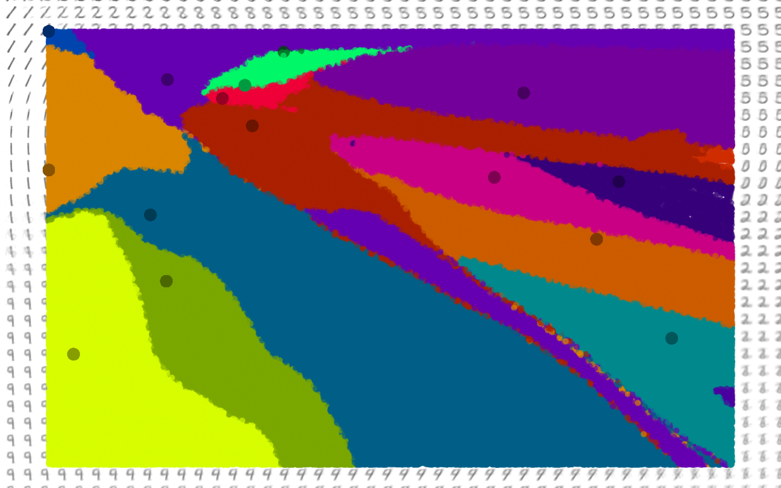
Another interesting thing you can do with this concept is to color points based on where they end up after being iterated repeatedly. This more clearly shows the regions which tend towards an individual "perfect" point.



Hopefully this slight detour was interesting. The next part of the series investigates some practical applications of autoencoders.

Technical details: The encoder consists of fully connected layers of these sizes: 784 (image input) --> 100 --> 50 --> 25 --> 2. The decoder contains the same layer sizes in reverse order. All nodes use the ReLU activation function (x when x > 0, 0 otherwise). For the purposes of clustering, the points are drawn using hidden layer 4's outputs under the activation function ln(x+1) when x > 0 and -ln(-x+1) otherwise. The first step of training was the creation of a deep belief network to use as encoder (by stacking successive restricted Boltzmann machines and using the contrastive divergence algorithm for each RBM to extract increasingly complex features), followed by flipping the weights to create the decoder, then fine-tuning using standard backpropagation. This would probably be considered somewhat out-of-date compared to current AE training techniques, but it was easier to learn and implement. All training and testing was done in Java without third-party libraries, for the sake of my own learning.

Disclaimer: This series attempts to explain how autoencoders work and provides my personal analysis of an autoencoder's behavior. It should be noted that I'm not an authority on this topic, as I have no formal machine learning or deep learning training. I've read up fairly heavily on the topic and implemented a several algorithms (including this one) from scratch, but the analysis I give in many of these descriptions will be my own and therefore should not be completely trusted. With that in mind, I still think this series shows off a pretty interesting ML algorithm and helps shed some light on its behavior.