Deep Autoencoder Demo - Decoder
Move your mouse to see how the mouse coordinates are decoded. Click to draw the image permanently.
This is the second part in a series discussing autoencoders. To understand what an autoencoder is, read the first part.
In the last demo, you learned the basics of how autoencoders work and saw an autoencoder perform dimensionality reduction, an important data analysis task. To do this, the autoencoder used its encoder to transform each image in a dataset into a point in 2D space. This demonstration shows the function of the other part of the autoencoder, the decoder.
While the encoder's job was to turn an image into coordinates, the decoder's job is to turn coordinates into an image. Specifically, the decoder tries to reconstruct the original image which the encoder mapped onto those coordinates, thus "decoding" the coordinates. When you move your mouse in this demo, your mouse coordinates are fed into the decoder and the resulting image is displayed in the top-left.
The decoder behaves much in the same way as the encoder, but in reverse. The areas where the encoder placed a certain number in the last demo will usually produce that number when fed into the decoder. The decoder can also explain some of the encoder's behavior. For example, in the last demo, the 2s (green dots) were split into two different, disconnected groups. If you inspect those same areas with the decoder, you can see why. See if you can find both groups!
As you may have noticed, the 2s in the larger group all have "loops" at the bottom. The smaller set of 2s in the top-left have no loops. This shows that the decision to split up the 2s is actually justified, since the two kinds of 2s are structurally different. The encoder thought the 2s without loops were more similar to 8s and slanted 1s, so it mapped them to a different area. As far as the encoder is concerned, this type of 2 could be a completely different number! For something which operates with no human knowledge, this is a justifiable conclusion. A similar splitting-up happens with the 5s and, to a certain extent, the 7s. See if you can find the extra groups of these numbers and tell what makes them different.
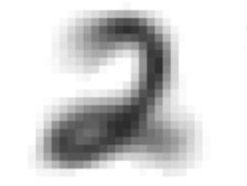
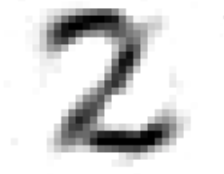
A 2 with a loop (left) vs. a 2 without a loop (right). These numbers are mapped to separate areas in 2D space by the encoder, as if they were different numbers.
Other transitions are less smooth, such as between 9s and 1s. These transitions involve a moment of chaos before one number turns into another. In the areas between such groups, the decoder comes up with ambiguous or nonsense images. These transitions could be interpreted as the encoder not necessarily thinking these numbers are similar, but being forced to place them adjacent to each other due to the restrictions of 2D space. It would be a lot to expect the encoder to have a smooth transition between every pair of adjacent numbers. However, it seems like the transition from 9 to 1 should be easy: just remove the left of the 9's loop and you're left with a vertical line. The only problem is that the line in a 9 is further right than the line in a 1. This exposes a weakness of this type of autoencoder: it doesn't deal well with translated shapes (shapes moved to different areas). To the autoencoder, a line in the middle and a line towards the right of the screen are totally dissimilar shapes, as they have no pixels in common. Other, more complicated autoencoder architectures have since solved this problem by treating translated shapes equally.
At this point, there are a few things which are important to point out. First of all, when an image is encoded and then decoded, the reconstructed image will almost definitely not be exactly the same as the original. If you encode an image of a 7, it will be encoded to the 2D area where most of the other 7s get encoded. When you decode those coordinates, you will get a similar, but different 7. If you encode an image of the capital letter B, it will probably get encoded to the area where the 8s are, since a B looks like an 8. When it is decoded, you will get an image of an 8, not a B. Any other image which isn't a number will similarly be turned into a number once encoded and decoded. It makes sense that the decoded image wouldn't be an exact copy of the original. If it was, that would mean this algorithm discovered a lossless compression algorithm which reduces the image size by 300x.
At this point, you understand the basics of how an autoencoder works and have seen both the encoder and the decoder in action. The next demo shows an application of autoencoders which requires both components: compression and denoising. As a side note if you are interested, this demo also explores some unrelated but interesting consequences of the decoder's imperfect reconstructions as you iterate the process over and over.
Technical details: The encoder consists of fully connected layers of these sizes: 784 (image input) --> 100 --> 50 --> 25 --> 2. The decoder contains the same layer sizes in reverse order. All nodes use the ReLU activation function (x when x > 0, 0 otherwise). For the purposes of clustering, the points are drawn using hidden layer 4's outputs under the activation function ln(x+1) when x > 0 and -ln(-x+1) otherwise. The first step of training was the creation of a deep belief network to use as encoder (by stacking successive restricted Boltzmann machines and using the contrastive divergence algorithm for each RBM to extract increasingly complex features), followed by flipping the weights to create the decoder, then fine-tuning using standard backpropagation. This would probably be considered somewhat out-of-date compared to current AE training techniques, but it was easier to learn and implement. All training and testing was done in Java without third-party libraries, for the sake of my own learning.
Disclaimer: This series attempts to explain how autoencoders work and provides my personal analysis of an autoencoder's behavior. It should be noted that I'm not an authority on this topic, as I have no formal machine learning or deep learning training. I've read up fairly heavily on the topic and implemented a several algorithms (including this one) from scratch, but the analysis I give in many of these descriptions will be my own and therefore should not be completely trusted. With that in mind, I still think this series shows off a pretty interesting ML algorithm and helps shed some light on its behavior.