Deep Autoencoder Demo - Encoder

This is a visualization of a deep autoencoder performing dimensionality reduction. Without understanding the technical details, all you need to know about an autoencoder is that it has an encoder and a decoder.

This autoencoder's encoder takes an image and converts it to a set of 2D coordinates. In this case, the images are 28x28 black-and-white images of handwritten digits, from 0 to 9. The encoder's goal is to assign coordinates so that similar images end up with coordinates near each other. For these images, you would expect the encoder to put images of the same number near each other.

This autoencoder's decoder takes a set of coordinates and attepts to reconstruct the image which the encoder mapped to those coordinates. The decoder will be explored later.

In this demonstration, the encoder is given images from a database of 60,000 handrwitten digits called MNIST. The image is then converted into 2D coordinates, and a circle is drawn at those coordinates. Since the MNIST database also labels each image with its actual number (0 to 9), we can color each circle based on the digit its image represents. Since the encoder's goal is to put similar images near each other, we would expect all the 1s to be near each other, the 2s to be near each other, and so on. This is represented visually by a clean separation of colors. This is actually happening live in your browser; the algorithm is randomly picking images and assigning them coordinates in the window above.

As the visualization runs and more points are drawn, you will begin to see that the colors are generally separated cleanly. For example, the 1s, represented by red dots, are concentrated almost entirely in the middle-left of the screen. This visualization runs quite slowly in browsers, however. To speed things up, here is what it looks like when 60,000 images have been mapped:



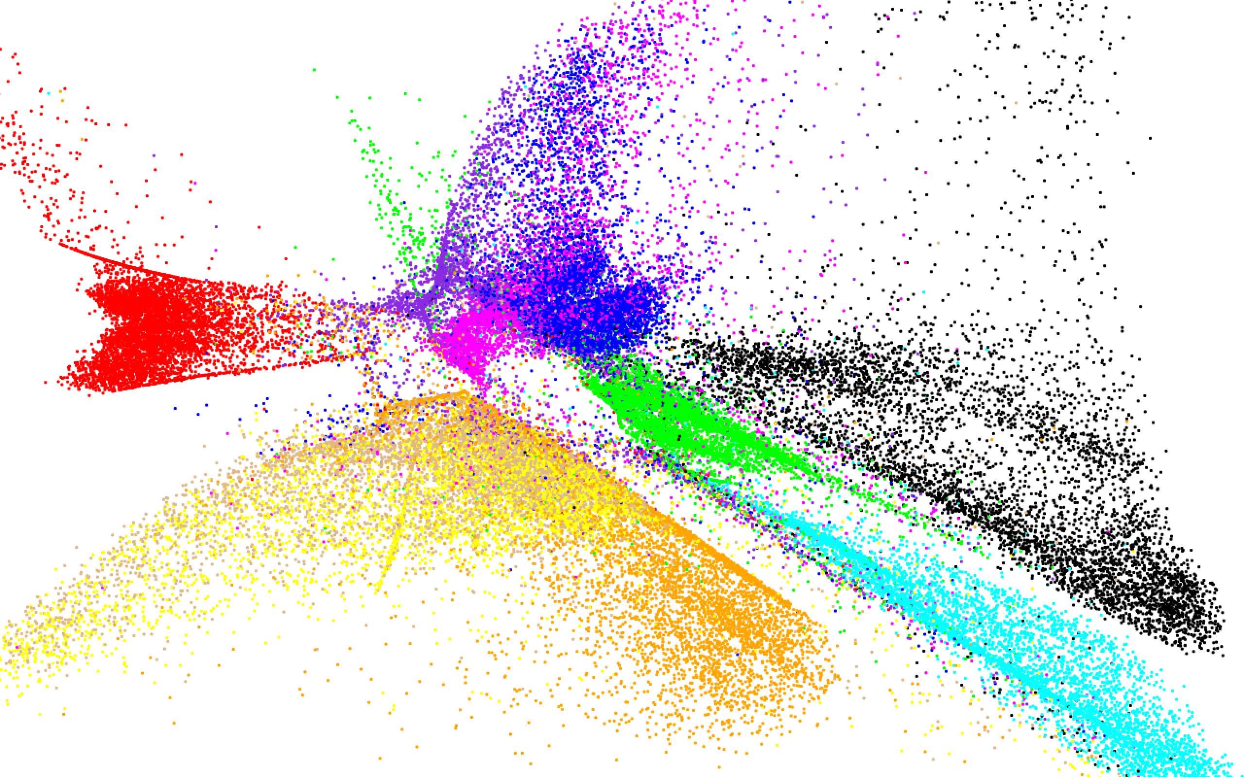
As you can see, the encoder does a pretty good job of grouping similar images. This is an example of an important aspect of data science called "dimensionality reduction". It is called dimensionality reduction because it turns each image from 784 pixels (784 dimensions) to just 2 dimensions in an information-preserving way. It is information-preserving because you can generally tell what an image looks like based on its 2D coordinate representation. Dimensionality reduction has many uses, from compression to data visualization.

So how were the encoder and decoder created? Essentially, the encoder and decoder both started out with random parameters which gave random results. Then, they were trained using the database of 60,000 images I mentioned earlier. During training, the encoder would encode an image to 2D coordinates, and the decoder would decode those coordinates in an attempt to recreate the original image. If the encoder had discovered an information-preserving transformation to 2D coordinates, the decoder would be able to reconstruct the image quite accurately. Otherwise, the encoder would improve itself by analyzing the decoder's failed reconstruction attempt (the actual analysis is accomplished with calculus). With each image, the encoder and decoder improved until a good information-preserving representation was found.

There are a few important things to note about this process. First of all, during training, the encoder and decoder never knew the label of the image they were working with. They never knew if the image was of a 1 or a 2 or a 3. They simply had to find a way to compress the image from 784 numbers to 2 numbers and reconstruct it fairly accurately. This brings me to my next point: this extreme degree of compression (784 to 2) is very difficult to accomplish, and relies heavily on patterns in the data. If this process was done with images of random noise, it would be nearly impossible to convert an image to a 2D point and then reconstruct the image from that. Instead, the algorithms had to notice patterns in the data. For example, the encoder might realize, "Hey, lots of these images are just a vertical line. If put all the vertical lines right here, then the decoder could turn all of these points into a vertical line." This allows accurate reconstructions and results in similar numbers being grouped together.

Autoencoders are quite good at dimensionality reduction. They do a better job than Principal Components Analysis (PCA), which is a very common dimensionality reduction algorithm. However, you can see that autoencoders are not perfect. For example, the encoder can't seem to tell the difference between 4s (yellow dots) and 9s (light tan dots) and as a result they are visually not very separated. Also, you might notice that there are two separate groups of 2s (green dots), although this actually isn't a bad thing and will be discussed in the next demo. Autoencoders have, in some respects, been surpassed by algorithms such as t-SNE in the domain of data visualization. However, they still have uses beyond data visualization due to the existence of the decoder and how the encoder interacts with the decoder. In the next demo, the decoder will be explored more.

Technical details: The encoder consists of fully connected layers of these sizes: 784 (image input) --> 100 --> 50 --> 25 --> 2. The decoder contains the same layer sizes in reverse order. All nodes use the ReLU activation function (x when x > 0, 0 otherwise). For the purposes of clustering, the points are drawn using hidden layer 4's outputs under the activation function ln(x+1) when x > 0 and -ln(-x+1) otherwise. The first step of training was the creation of a deep belief network to use as encoder (by stacking successive restricted Boltzmann machines and using the contrastive divergence algorithm for each RBM to extract increasingly complex features), followed by flipping the weights to create the decoder, then fine-tuning using standard backpropagation. This would probably be considered somewhat out-of-date compared to current AE training techniques, but it was easier to learn and implement. All training and testing was done in Java without third-party libraries, for the sake of my own learning. The images being used for the browser demo come from the MNIST test set, but the images used in the larger image come from the MNIST training set. The test data is smaller and easier to transmit for the demo, but I used training data to show the finished product because there were more images in the training set. Since this is an unsupervised task, there's no issue with using the training set to show off the results.

Disclaimer: This series attempts to explain how autoencoders work and provides my personal analysis of an autoencoder's behavior. It should be noted that I'm not an authority on this topic, as I have no formal machine learning or deep learning training. I've read up fairly heavily on the topic and implemented a several algorithms (including this one) from scratch, but the analysis I give in many of these descriptions will be my own and therefore should not be completely trusted. With that in mind, I still think this series shows off a pretty interesting ML algorithm and helps shed some light on its behavior.